If you’ve ever seen me digging through nested folders or dumpster-diving for that one CSV file, you know it’s just a typical day in the life of a data wrangler; usually, I just feel like a trash panda. Half the columns are missing, some files won’t even open, and everything else is misnamed: chaos, pure and simple. That’s exactly why I built trashpanda: to help me tame messy file systems, clean up unruly data, beautify plots, manage colour palettes, and automate the little tasks that normally make me want to throw my computer into a real dumpster fire.
Installation
You can install the development version of trashpanda from GitHub with:
devtools::install_github("colebaril/trashpanda")Example
Themes and Palettes
In the following example, theme_cole() is used to alter thematic elements of the plot and scale_cwb() is used to apply my custom colour palettes. I also use the add_caption_cwb() function to automatically insert a caption that is pre-formatted with icons and social media tags. You can easily flip to dark mode!
require(pacman)
p_load(trashpanda, ggplot2, palmerpenguins)

ggplot(penguins, aes(flipper_length_mm, bill_length_mm, fill = species, group = species)) +
  geom_point(shape = 21) +
  geom_smooth(aes(colour = species), se = FALSE, method = "lm") +
  scale_cwb(name = "Species", palette = "arcane_flame", type = "d", aesthetics = "fill") +
  scale_cwb(name = "Species", palette = "arcane_flame", type = "d", aesthetics = "colour") +
  theme_cole(show_axis_lines = c("bottom", "left"), remove_grid = TRUE) +
  labs(title = "Palmer Penguin Bill Length \nvs. Flipper Length", x = "Flipper Length (mm)", y = "Bill Length (mm)") +
add_caption_cwb(type = "plot") 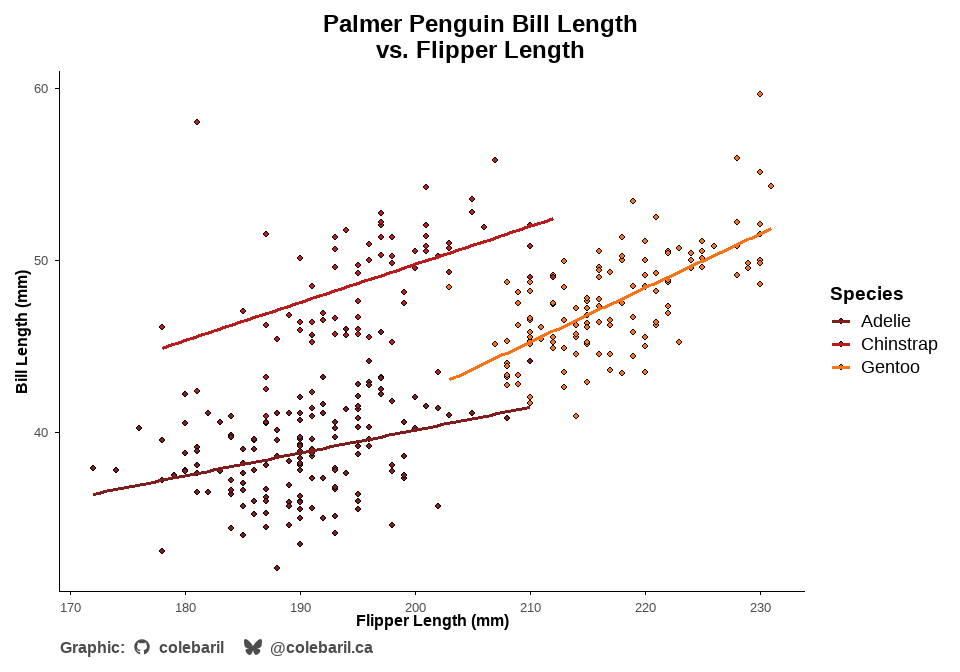
ggplot(penguins, aes(flipper_length_mm, bill_length_mm, fill = species, group = species)) +
  geom_point(shape = 21) +
  geom_smooth(aes(colour = species), se = FALSE, method = "lm") +
  scale_cwb(name = "Species", palette = "arcane_flame", type = "d", aesthetics = "fill") +
  scale_cwb(name = "Species", palette = "arcane_flame", type = "d", aesthetics = "colour") +
  theme_cole(show_axis_lines = c("bottom", "left"), remove_grid = TRUE, dark = TRUE) +
  labs(title = "Palmer Penguin Bill Length \nvs. Flipper Length", x = "Flipper Length (mm)", y = "Bill Length (mm)") +
add_caption_cwb(type = "plot") 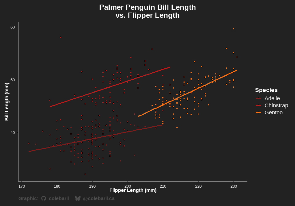
Data Cleaning
In this example, clean_data() is used to standardize column names, trim white space, convert empty columns to true NAs, and flags outliers for any numeric columns using robust means.
df <- tibble::tibble(
  "First Name" = c(" Alice ", "Bob", "", "CHARLIE", "dave", "Eve", NA, "Bob", "Bob"),
  "Last Name" = c("Smith", "Jones", "O'Neil", "Brown", "Miller", "O'Brien", "", "Jones", "Jones"),
  "Score" = c(10, 5000, 15, 20, 12, -999, 14, 5000, 5000),
  "Enrollment Date" = c("2025-01-01", "20241215", "2025/02/01", "", NA, "01-03-2025", "2025-01-01", "2024-12-15", "2024-12-15"),
  "Grade" = c("A", "b", "C", "A", "B", "", "A", "b", "b"),
  "Comments!" = c("Good", " Excellent ", "", "Needs work", NA, "Good!", "Average", " Excellent ", " Excellent "),
  "EmptyCol" = c(NA, NA, NA, NA, NA, NA, NA, NA, NA)
)

print(df)
#> # A tibble: 9 × 7
#>   `First Name` `Last Name` Score `Enrollment Date` Grade `Comments!`   EmptyCol
#>   <chr>        <chr>       <dbl> <chr>             <chr> <chr>         <lgl>
#> 1 " Alice "    "Smith"        10 "2025-01-01"      "A"   "Good"        NA
#> 2 "Bob"        "Jones"      5000 "20241215"        "b"   " Excellent " NA
#> 3 ""           "O'Neil"       15 "2025/02/01"      "C"   ""            NA
#> 4 "CHARLIE"    "Brown"        20 ""                "A"   "Needs work"  NA
#> 5 "dave"       "Miller"       12  <NA>             "B"    <NA>         NA
#> 6 "Eve"        "O'Brien"    -999 "01-03-2025"      ""    "Good!"       NA
#> 7  <NA>        ""             14 "2025-01-01"      "A"   "Average"     NA
#> 8 "Bob"        "Jones"      5000 "2024-12-15"      "b"   " Excellent " NA
#> 9 "Bob"        "Jones"      5000 "2024-12-15"      "b"   " Excellent " NA

clean_data(df, trim_chars = TRUE, empty_to_na = TRUE, flag_outliers = TRUE)
#> # A tibble: 8 × 8
#>   first_name last_name score enrollment_date grade comments   empty_col
#>   <chr>      <chr>     <dbl> <chr>           <chr> <chr>      <lgl>
#> 1 Alice      Smith        10 2025-01-01      A     Good       NA
#> 2 Bob        Jones      5000 20241215        b     Excellent  NA
#> 3 <NA>       O'Neil       15 2025/02/01      C     <NA>       NA
#> 4 CHARLIE    Brown        20 <NA>            A     Needs work NA
#> 5 dave       Miller       12 <NA>            B     <NA>       NA
#> 6 Eve        O'Brien    -999 01-03-2025      <NA>  Good!      NA
#> 7 <NA>       <NA>         14 2025-01-01      A     Average    NA
#> 8 Bob        Jones      5000 2024-12-15      b     Excellent  NA
#> # ℹ 1 more variable: score_outlier_flag <lgl>
Read Multiple Files
When I’m wrangling messy data across multiple folders and files, read_data_tree() is my go-to helper. It recursively searches a folder for files, reads them safely (even if some files are malformed), and combines everything into a single tidy tibble. Excel sheets with mixed types? No problem — all columns are safely coerced so you won’t get errors on binding rows. You can also select specific sheets by name or pattern, filter by extensions, and enforce consistent columns.
# Read all CSV files in nested "Test" folder, ignore "extra folder"
results_csv <- read_data_tree(
  path = "C:/File_Path",
  ext = "csv",
  exclude = "extra folder",
  reader = readr::read_csv,
  cols = c("id", "value", "date")
)

# Read all sheets in all Excel files containing "Data" in the sheet name
results_excel <- read_data_tree(
  path = "C:/File_Path",
  ext = "xlsx",
  reader = readxl::read_excel,
  sheet_pattern = "Data",
  cols = c("a", "b", "c")
)
Find tables
Find tables within multiple Excel files and sheets regardless of where the table is within the sheet with the extract_table() function. In the example below, every excel file in the base directory and below is read. Within each Excel file, tables that start with Sample ID are located and data from those tables is combined into one tibble. It automatically detects when the sample ends or you can specify an ending column. You can also specify the number of empty rows allowed before the table is deemed to have ended. See extract_table() documentation for more details.
read_data_tree(
  path = here(),
  ext = "xlsx",
  recursive = TRUE,
  reader = extract_table,
  start_column = "Sample ID",
  table_mode = "all",
  safely = TRUE,
  id_cols = FALSE
)
Citing Packages
Using the trashpanda::cite_packages() function, you can easily cite all packages used in your script or file, choosing between R Markdown output or plain text options.
cite_packages(format = "rmd")Horst AM, Hill AP, Gorman KB (2020). palmerpenguins: Palmer Archipelago (Antarctica) penguin data. doi:10.5281/zenodo.3960218 https://doi.org/10.5281/zenodo.3960218, R package version 0.1.0, https://allisonhorst.github.io/palmerpenguins/.
Wickham H (2016). ggplot2: Elegant Graphics for Data Analysis. Springer-Verlag New York. ISBN 978-3-319-24277-4, https://ggplot2.tidyverse.org.
Baril C (2026). trashpanda: Cole’s personal collection of R functions, themes, and palettes. R package version 0.0.1, commit 14145a48ec656cb89aa5ca8a60aeb12a5c89b085, https://github.com/colebaril/trashpanda.
Rinker TW, Kurkiewicz D (2018). pacman: Package Management for R. version 0.5.0, http://github.com/trinker/pacman.