require(pacman)
p_load(tidytuesdayR, magick, tidyverse, janitor, here, trashpanda, glue, ggtext, ggside, scales, ggridges, ggtext, ggview)Brazilian Companies
business
finance
brazil
What types of firms control the most capital?
Load Packages
Load Data
tuesdata <- tidytuesdayR::tt_load('2026-01-27')
companies <- tuesdata$companies
legal_nature <- tuesdata$legal_nature
qualifications <- tuesdata$qualifications
size <- tuesdata$size
Data Cleaning
lorenz_df <- companies |>
  filter(!is.na(capital_stock),
         capital_stock > 0,
         !is.na(owner_qualification)) |>
  group_by(owner_qualification) |>
  ungroup() |>

  group_by(owner_qualification) |>
  arrange(capital_stock, .by_group = TRUE) |>
  mutate(
    firm_rank   = row_number(),
    firm_share  = firm_rank / n(),
    capital_cum = cumsum(capital_stock),
    capital_share = capital_cum / sum(capital_stock)
  ) |>
  ungroup()

owner_order <- lorenz_df %>%
  group_by(owner_qualification) %>%
  summarise(
    capital_top_1pct = capital_share[which.min(abs(firm_share - 0.99))]
  ) %>%
  arrange(capital_top_1pct) %>%
  pull(owner_qualification)

lorenz_df <- lorenz_df %>%
  mutate(
    owner_qualification = factor(owner_qualification,
                                 levels = owner_order)
  )
Share of Capital
Lorenz Plot
ggplot(
  lorenz_df,
  aes(firm_share, capital_share, colour = owner_qualification)) +
  geom_line(linewidth = 1.3, alpha = 0.95) +
  geom_abline(
    slope = 1,
    intercept = 0,
    linetype = "dashed",
    colour = "grey60",
    linewidth = 0.8) +
  cwb::scale_cwb("discrete_21", type = "d", aesthetics = "colour", name = "Owner qualification") +
  scale_x_continuous(
    labels = percent_format(),
    expand = c(0, 0)) +
  scale_y_continuous(
    labels = percent_format(),
    expand = c(0, 0)) +
  labs(
    title = "A Small Share of Firms Controls Most Declared Capital",
    subtitle = "Cumulative share capital by leadership role for Brazilian companies",
    x = "Cumulative share of companies",
    y = "Cumulative share of total declared capital") +
    theme_cole(remove_grid = TRUE) +
    add_caption_cwb()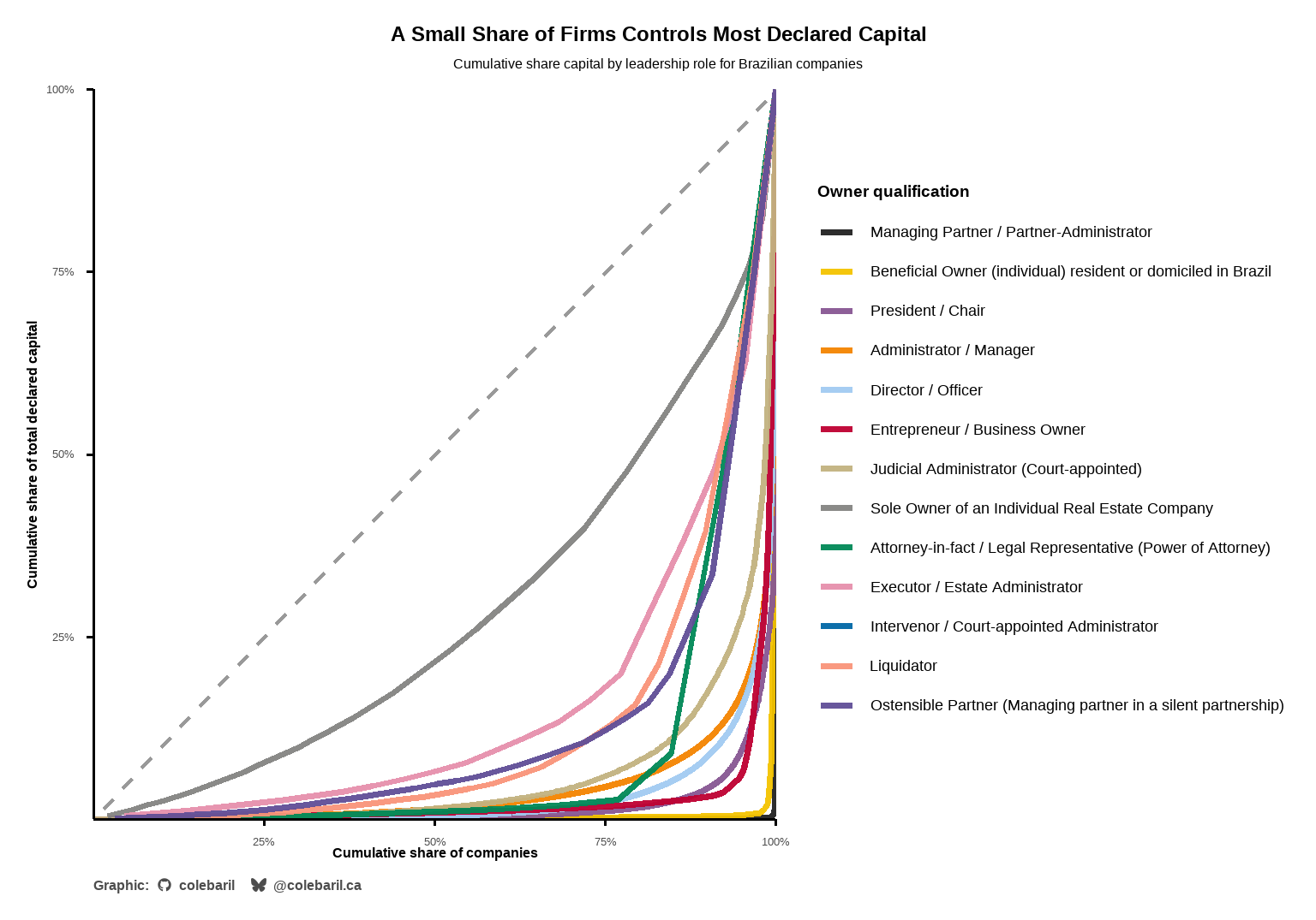
Ridgeline Plot
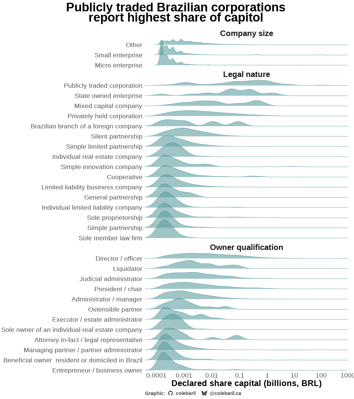
companies_long <- companies |>
  select(legal_nature, owner_qualification, company_size, capital_stock) |>
  pivot_longer(!capital_stock, names_to = "group", values_to = "category") |>
  mutate(
    group = str_replace(group, "_", " "),
    group = str_to_sentence(group),
    category = str_remove_all(category, "\\(.*?\\)"),
    category = str_trim(category),
    category = str_replace(category, "-", " "),
    category = str_to_sentence(category),
    category = str_replace(category, "llc", "LLC"),
    category = str_replace(category, "brazil", "Brazil")
  ) |>
  mutate(capital_stock = capital_stock / 1000000000) |>
  mutate(n = n(), .by = c(group, category)) |>
  filter(n >= 5) |>
  mutate(y = n_distinct(category), .by = group)

summary_data <- companies_long |>
  summarise(med = median(capital_stock),
            .by = c(group, category)) |>
  arrange(desc(med))

companies_long$category <- factor(companies_long$category, levels = summary_data$category)


plot2 <- ggplot() +
  geom_density_ridges(
    data = companies_long,
    mapping = aes(x = capital_stock, y = category),
    fill = "cadetblue",
    colour = "cadetblue",
    alpha = 0.6) +
  facet_wrap(~group, scales = "free_y", space = "free_y") +
  scale_x_log10(limits = c(0.00005, 1000),
                breaks = c(0.0001, 0.001, 0.01, 0.1, 1, 10, 100, 1000),
                labels = function(x) format(x, scientific = FALSE, drop0trailing = TRUE)) +
      scale_y_discrete(
        limits = rev
      ) +
  labs(
    x = "Declared share capital (billions, BRL)", y = NULL,
    title = "Publicly traded Brazilian corporations\nreport highest share of capitol") +
  coord_cartesian(expand = FALSE, clip = "off") +
  theme_cole(base_size = 20, dark = FALSE, remove_grid = TRUE, show_axis_lines = "none") +
  theme(
    plot.margin = margin(10, 20, 10, 10),
    axis.title.x = element_text(margin = margin(t = 5, b = 10)),
    axis.text.y = element_text(margin = margin(r = 0)),
    strip.text = element_text(size = 15 * 1.3)) +
    add_caption_cwb()

# Save and display images
current_dir <- dirname(knitr::current_input())
plot_name <- "brazil_ridgeline.png"

ggsave(plot = plot2,
       dpi = "screen",
       width = 16,
       height = 18,
       device = ragg::agg_png,
       filename = file.path(current_dir, plot_name))


img <- image_read(file.path(current_dir, plot_name))

img_card <- image_scale(img, "1200x675")
img_card <- image_extent(
  img_card,
  geometry = "1200x675",
  gravity = "center"
)

# Save as card preview
image_write(img_card, path = file.path(current_dir, "preview.png"))

knitr::include_graphics(
  file.path(current_dir, plot_name)
)
References
trashpanda::cite_packages(format = "rmd")Domin I (2025). ggview: ‘ggplot2’ Picture Previewer. doi:10.32614/CRAN.package.ggview https://doi.org/10.32614/CRAN.package.ggview, R package version 0.2.2, https://CRAN.R-project.org/package=ggview.
Wilke C (2025). ggridges: Ridgeline Plots in ‘ggplot2’. doi:10.32614/CRAN.package.ggridges https://doi.org/10.32614/CRAN.package.ggridges, R package version 0.5.7, https://CRAN.R-project.org/package=ggridges.
Wickham H, Pedersen T, Seidel D (2025). scales: Scale Functions for Visualization. doi:10.32614/CRAN.package.scales https://doi.org/10.32614/CRAN.package.scales, R package version 1.4.0, https://CRAN.R-project.org/package=scales.
Landis J (2025). ggside: Side Grammar Graphics. doi:10.32614/CRAN.package.ggside https://doi.org/10.32614/CRAN.package.ggside, R package version 0.4.1, https://CRAN.R-project.org/package=ggside.
Wilke C, Wiernik B (2022). ggtext: Improved Text Rendering Support for ‘ggplot2’. doi:10.32614/CRAN.package.ggtext https://doi.org/10.32614/CRAN.package.ggtext, R package version 0.1.2, https://CRAN.R-project.org/package=ggtext.
Hester J, Bryan J (2024). glue: Interpreted String Literals. doi:10.32614/CRAN.package.glue https://doi.org/10.32614/CRAN.package.glue, R package version 1.8.0, https://CRAN.R-project.org/package=glue.
Baril C (????). trashpanda: Cole’s Personal Collection of R Functions, Themes, and Palettes. R package version 0.0.1, https://colebaril.github.io/trashpanda/.
Müller K (2025). here: A Simpler Way to Find Your Files. doi:10.32614/CRAN.package.here https://doi.org/10.32614/CRAN.package.here, R package version 1.0.2, https://CRAN.R-project.org/package=here.
Firke S (2024). janitor: Simple Tools for Examining and Cleaning Dirty Data. doi:10.32614/CRAN.package.janitor https://doi.org/10.32614/CRAN.package.janitor, R package version 2.2.1, https://CRAN.R-project.org/package=janitor.
Grolemund G, Wickham H (2011). “Dates and Times Made Easy with lubridate.” Journal of Statistical Software, 40(3), 1-25. https://www.jstatsoft.org/v40/i03/.
Wickham H (2025). forcats: Tools for Working with Categorical Variables (Factors). doi:10.32614/CRAN.package.forcats https://doi.org/10.32614/CRAN.package.forcats, R package version 1.0.1, https://CRAN.R-project.org/package=forcats.
Wickham H (2025). stringr: Simple, Consistent Wrappers for Common String Operations. doi:10.32614/CRAN.package.stringr https://doi.org/10.32614/CRAN.package.stringr, R package version 1.6.0, https://CRAN.R-project.org/package=stringr.
Wickham H, François R, Henry L, Müller K, Vaughan D (2023). dplyr: A Grammar of Data Manipulation. doi:10.32614/CRAN.package.dplyr https://doi.org/10.32614/CRAN.package.dplyr, R package version 1.1.4, https://CRAN.R-project.org/package=dplyr.
Wickham H, Henry L (2026). purrr: Functional Programming Tools. doi:10.32614/CRAN.package.purrr https://doi.org/10.32614/CRAN.package.purrr, R package version 1.2.1, https://CRAN.R-project.org/package=purrr.
Wickham H, Hester J, Bryan J (2025). readr: Read Rectangular Text Data. doi:10.32614/CRAN.package.readr https://doi.org/10.32614/CRAN.package.readr, R package version 2.1.6, https://CRAN.R-project.org/package=readr.
Wickham H, Vaughan D, Girlich M (2025). tidyr: Tidy Messy Data. doi:10.32614/CRAN.package.tidyr https://doi.org/10.32614/CRAN.package.tidyr, R package version 1.3.2, https://CRAN.R-project.org/package=tidyr.
Müller K, Wickham H (2026). tibble: Simple Data Frames. doi:10.32614/CRAN.package.tibble https://doi.org/10.32614/CRAN.package.tibble, R package version 3.3.1, https://CRAN.R-project.org/package=tibble.
Wickham H (2016). ggplot2: Elegant Graphics for Data Analysis. Springer-Verlag New York. ISBN 978-3-319-24277-4, https://ggplot2.tidyverse.org.
Wickham H, Averick M, Bryan J, Chang W, McGowan LD, François R, Grolemund G, Hayes A, Henry L, Hester J, Kuhn M, Pedersen TL, Miller E, Bache SM, Müller K, Ooms J, Robinson D, Seidel DP, Spinu V, Takahashi K, Vaughan D, Wilke C, Woo K, Yutani H (2019). “Welcome to the tidyverse.” Journal of Open Source Software, 4(43), 1686. doi:10.21105/joss.01686 https://doi.org/10.21105/joss.01686.
Ooms J (2025). magick: Advanced Graphics and Image-Processing in R. doi:10.32614/CRAN.package.magick https://doi.org/10.32614/CRAN.package.magick, R package version 2.9.0, https://CRAN.R-project.org/package=magick.
Harmon J, Hughes E (2025). tidytuesdayR: Access the Weekly ‘TidyTuesday’ Project Dataset. doi:10.32614/CRAN.package.tidytuesdayR https://doi.org/10.32614/CRAN.package.tidytuesdayR, R package version 1.2.1, https://CRAN.R-project.org/package=tidytuesdayR.
Rinker TW, Kurkiewicz D (2018). pacman: Package Management for R. version 0.5.0, http://github.com/trinker/pacman.