require(pacman)
p_load(trashpanda, magick, tidytuesdayR, tidyverse, janitor, tidytext, extrafont, here,
sf, rnaturalearth, rnaturalearthdata, patchwork, ggflags, gt, gtExtras)Passport Power
geography
maps
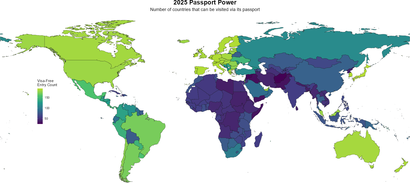
Which country has the most powerful passport?
Load Packages
Load Data
tuesdata <- tidytuesdayR::tt_load('2025-09-09')

country_lists <- tuesdata$country_lists
rank_by_year <- tuesdata$rank_by_year

rank_by_year <- rank_by_year |>
      mutate(code = case_when(country == "Namibia" ~ "NA",
                            .default = code))
World Map
world <- rnaturalearth::ne_countries(scale = 50) |>
  filter(admin != "Antarctica") |>
  select(admin, iso_a2) |>
  left_join(rank_by_year, by = c("iso_a2" = "code"))


plot <- world |>
  filter(year == "2025") |>
  ggplot() +
  geom_sf(aes(fill = visa_free_count), colour = "black", linewidth = 0.2) +
  scale_fill_viridis_c("Visa-Free\nEntry Count", end = 0.9) +
  theme_void(base_size = 15) +
  theme(panel.border = element_blank(),
        panel.grid.major = element_blank(),
        axis.text = element_blank(),
        axis.ticks = element_blank(),
        plot.title = element_text(size = 25, face = "bold", hjust = 0.5),
        plot.subtitle = element_text(size = 18, hjust = 0.5),
        legend.position = "inside",
        legend.position.inside = c(0.15, 0.50),
        legend.key.width = unit(0.75, "cm"),
        legend.key.height = unit(1, "cm")
        ) +
  labs(title = "2025 Passport Power",
       subtitle = "Number of countries that can be visited via its passport")

# Save and display images
current_dir <- dirname(knitr::current_input())
plot_name <- "passport_power.png"

ggsave(plot = plot,
       dpi = "screen",
       width = 25,
       height = 25,
       device = ragg::agg_png,
       filename = file.path(current_dir, plot_name))


# Read the big plot
img <- image_read(file.path(current_dir, plot_name)) |> image_trim()

image_write(img, file.path(current_dir, plot_name))

# Force 16:9 aspect ratio with minimal padding
# Target size: 1200x675 px (16:9)
img_card <- image_scale(img, "1200x675")           # scale to fit inside 16:9
img_card <- image_extent(
  img_card,
  geometry = "1200x675",
  gravity = "center"
)

# Save as card preview
image_write(img_card, path = file.path(current_dir, "preview.png"))

knitr::include_graphics(
  file.path(current_dir, plot_name)
)
Most Powerful Passports
t <- world |>
  st_drop_geometry() |>
  filter(!year %in% c("2007", "2009")) |>
  select(iso_a2, country, visa_free_count, year) |>
  arrange(year, .by = country) |>
  reframe(visa_free_count_list = list(visa_free_count),
          .by = country) |>
  drop_na(country)

world |>
  st_drop_geometry() |>
  filter(year %in% c("2025", "2024")) |>
  select(iso_a2, country, visa_free_count, year) |>
  pivot_wider(names_from = year, values_from = visa_free_count) |>
  relocate(`2025`, .before = `2024`) |>
  mutate(change = `2025` - `2024`) |>
  left_join(t, by = "country") |>
  arrange(desc(`2025`)) |>
  head(10) |>
  gt() |>
  fmt_flag(columns = iso_a2) |>
  cols_add(dir = ifelse(`2024` < `2025`, "arrow-up", "arrow-down")) |>
  fmt_icon(
    columns = dir,
    fill_color = c("arrow-up" = "green", "arrow-down" = "red")
  ) |>
  cols_hide(c(`2025`, `2024`)) |>
  cols_move(dir, after = change) |>
  gt_plt_sparkline(column = visa_free_count_list,
                   fig_dim = c(20, 30)) |>
  cols_label(iso_a2 = "",
             dir = "",
             country = "Country",
             change = "2024-2025 Change",
             visa_free_count_list = "Visa Free Count \nOver Time (2006-2025)") |>
  cols_align(columns = 5, align = "center") |>
  tab_header(
    title = md("**Top 10 Most Powerful Passports**")
  ) |>
  opt_table_font(font = "Courier New") |>
    tab_options(
    table.background.color = "white"
)| Top 10 Most Powerful Passports | ||||
| Country | 2024-2025 Change | Visa Free Count Over Time (2006-2025) | ||
|---|---|---|---|---|
| Singapore | -1 | |||
| South Korea | -3 | |||
| Japan | -4 | |||
| Spain | -5 | |||
| Italy | -5 | |||
| Ireland | -3 | |||
| Germany | -5 | |||
| Finland | -4 | |||
| Denmark | -3 | |||
| Sweden | -5 | |||
Least Powerful Passports
t <- world |>
  st_drop_geometry() |>
  filter(!year %in% c("2007", "2009")) |>
  select(iso_a2, country, visa_free_count, year) |>
  arrange(year, .by = country) |>
  reframe(visa_free_count_list = list(visa_free_count),
          .by = country) |>
  drop_na(country)

world |>
  st_drop_geometry() |>
  filter(year %in% c("2025", "2024")) |>
  select(iso_a2, country, visa_free_count, year) |>
  pivot_wider(names_from = year, values_from = visa_free_count) |>
  relocate(`2025`, .before = `2024`) |>
  mutate(change = `2025` - `2024`) |>
  left_join(t, by = "country") |>
  arrange(`2025`) |>
  head(10) |>
  gt() |>
  fmt_flag(columns = iso_a2) |>
  cols_add(dir = ifelse(`2024` < `2025`, "arrow-up", "arrow-down")) |>
  fmt_icon(
    columns = dir,
    fill_color = c("arrow-up" = "green", "arrow-down" = "red")
  ) |>
  cols_hide(c(`2025`, `2024`)) |>
  cols_move(dir, after = change) |>
  gt_plt_sparkline(column = visa_free_count_list,
                   fig_dim = c(20, 30)) |>
  cols_label(iso_a2 = "",
             dir = "",
             country = "Country",
             change = "2024-2025 Change",
             visa_free_count_list = "Visa Free Count \nOver Time (2006-2025)") |>
  cols_align(columns = 5, align = "center") |>
  tab_header(
    title = md("**Top 10 Least Powerful Passports**")
  ) |>
  opt_table_font(font = "Courier New") |>
  tab_options(
    table.background.color = "white"
)| Top 10 Least Powerful Passports | ||||
| Country | 2024-2025 Change | Visa Free Count Over Time (2006-2025) | ||
|---|---|---|---|---|
| Afghanistan | -3 | |||
| Syria | -2 | |||
| Iraq | -1 | |||
| Yemen | -3 | |||
| Somalia | -4 | |||
| Pakistan | -2 | |||
| Nepal | -2 | |||
| Libya | -2 | |||
| Palestinian Territory | -1 | |||
| Eritrea | -4 | |||
References
trashpanda::cite_packages(format = "rmd")Mock T (2026). gtExtras: Extending ‘gt’ for Beautiful HTML Tables. doi:10.32614/CRAN.package.gtExtras https://doi.org/10.32614/CRAN.package.gtExtras, R package version 0.6.2, https://CRAN.R-project.org/package=gtExtras.
Iannone R, Cheng J, Schloerke B, Haughton S, Hughes E, Lauer A, François R, Seo J, Brevoort K, Roy O (2026). gt: Easily Create Presentation-Ready Display Tables. doi:10.32614/CRAN.package.gt https://doi.org/10.32614/CRAN.package.gt, R package version 1.3.0, https://CRAN.R-project.org/package=gt.
Auguie B, Goldie J, Thériault R (2023). ggflags: Plot flags of the world in ggplot2. R package version 0.0.4, https://github.com/jimjam-slam/ggflags.
Pedersen T (2025). patchwork: The Composer of Plots. doi:10.32614/CRAN.package.patchwork https://doi.org/10.32614/CRAN.package.patchwork, R package version 1.3.2, https://CRAN.R-project.org/package=patchwork.
South A, Michael S, Massicotte P (2024). rnaturalearthdata: World Vector Map Data from Natural Earth Used in ‘rnaturalearth’. doi:10.32614/CRAN.package.rnaturalearthdata https://doi.org/10.32614/CRAN.package.rnaturalearthdata, R package version 1.0.0, https://CRAN.R-project.org/package=rnaturalearthdata.
Massicotte P, South A (2026). rnaturalearth: World Map Data from Natural Earth. doi:10.32614/CRAN.package.rnaturalearth https://doi.org/10.32614/CRAN.package.rnaturalearth, R package version 1.2.0, https://CRAN.R-project.org/package=rnaturalearth.
Pebesma E, Bivand R (2023). Spatial Data Science: With applications in R. Chapman and Hall/CRC. doi:10.1201/9780429459016 https://doi.org/10.1201/9780429459016, https://r-spatial.org/book/.
Pebesma E (2018). “Simple Features for R: Standardized Support for Spatial Vector Data.” The R Journal, 10(1), 439-446. doi:10.32614/RJ-2018-009 https://doi.org/10.32614/RJ-2018-009, https://doi.org/10.32614/RJ-2018-009.
Müller K (2025). here: A Simpler Way to Find Your Files. doi:10.32614/CRAN.package.here https://doi.org/10.32614/CRAN.package.here, R package version 1.0.2, https://CRAN.R-project.org/package=here.
Chang W (2025). extrafont: Tools for Using Fonts. doi:10.32614/CRAN.package.extrafont https://doi.org/10.32614/CRAN.package.extrafont, R package version 0.20, https://CRAN.R-project.org/package=extrafont.
Silge J, Robinson D (2016). “tidytext: Text Mining and Analysis Using Tidy Data Principles in R.” JOSS, 1(3). doi:10.21105/joss.00037 https://doi.org/10.21105/joss.00037, http://dx.doi.org/10.21105/joss.00037.
Firke S (2024). janitor: Simple Tools for Examining and Cleaning Dirty Data. doi:10.32614/CRAN.package.janitor https://doi.org/10.32614/CRAN.package.janitor, R package version 2.2.1, https://CRAN.R-project.org/package=janitor.
Grolemund G, Wickham H (2011). “Dates and Times Made Easy with lubridate.” Journal of Statistical Software, 40(3), 1-25. https://www.jstatsoft.org/v40/i03/.
Wickham H (2025). forcats: Tools for Working with Categorical Variables (Factors). doi:10.32614/CRAN.package.forcats https://doi.org/10.32614/CRAN.package.forcats, R package version 1.0.1, https://CRAN.R-project.org/package=forcats.
Wickham H (2025). stringr: Simple, Consistent Wrappers for Common String Operations. doi:10.32614/CRAN.package.stringr https://doi.org/10.32614/CRAN.package.stringr, R package version 1.6.0, https://CRAN.R-project.org/package=stringr.
Wickham H, François R, Henry L, Müller K, Vaughan D (2023). dplyr: A Grammar of Data Manipulation. doi:10.32614/CRAN.package.dplyr https://doi.org/10.32614/CRAN.package.dplyr, R package version 1.1.4, https://CRAN.R-project.org/package=dplyr.
Wickham H, Henry L (2026). purrr: Functional Programming Tools. doi:10.32614/CRAN.package.purrr https://doi.org/10.32614/CRAN.package.purrr, R package version 1.2.1, https://CRAN.R-project.org/package=purrr.
Wickham H, Hester J, Bryan J (2025). readr: Read Rectangular Text Data. doi:10.32614/CRAN.package.readr https://doi.org/10.32614/CRAN.package.readr, R package version 2.1.6, https://CRAN.R-project.org/package=readr.
Wickham H, Vaughan D, Girlich M (2025). tidyr: Tidy Messy Data. doi:10.32614/CRAN.package.tidyr https://doi.org/10.32614/CRAN.package.tidyr, R package version 1.3.2, https://CRAN.R-project.org/package=tidyr.
Müller K, Wickham H (2026). tibble: Simple Data Frames. doi:10.32614/CRAN.package.tibble https://doi.org/10.32614/CRAN.package.tibble, R package version 3.3.1, https://CRAN.R-project.org/package=tibble.
Wickham H (2016). ggplot2: Elegant Graphics for Data Analysis. Springer-Verlag New York. ISBN 978-3-319-24277-4, https://ggplot2.tidyverse.org.
Wickham H, Averick M, Bryan J, Chang W, McGowan LD, François R, Grolemund G, Hayes A, Henry L, Hester J, Kuhn M, Pedersen TL, Miller E, Bache SM, Müller K, Ooms J, Robinson D, Seidel DP, Spinu V, Takahashi K, Vaughan D, Wilke C, Woo K, Yutani H (2019). “Welcome to the tidyverse.” Journal of Open Source Software, 4(43), 1686. doi:10.21105/joss.01686 https://doi.org/10.21105/joss.01686.
Harmon J, Hughes E (2025). tidytuesdayR: Access the Weekly ‘TidyTuesday’ Project Dataset. doi:10.32614/CRAN.package.tidytuesdayR https://doi.org/10.32614/CRAN.package.tidytuesdayR, R package version 1.2.1, https://CRAN.R-project.org/package=tidytuesdayR.
Ooms J (2025). magick: Advanced Graphics and Image-Processing in R. doi:10.32614/CRAN.package.magick https://doi.org/10.32614/CRAN.package.magick, R package version 2.9.0, https://CRAN.R-project.org/package=magick.
Baril C (????). trashpanda: Cole’s Personal Collection of R Functions, Themes, and Palettes. R package version 0.0.1, https://colebaril.github.io/trashpanda/.
Rinker TW, Kurkiewicz D (2018). pacman: Package Management for R. version 0.5.0, http://github.com/trinker/pacman.